Lab Report - [Lab Name]

Introduction

In this lab, the objective is to utilize code provided to

Procedures

A.1) What happens to the overall signal when harmonics are added?
When I run the sections that have more harmonics added the sound played is not only way louder but also has a higher pitch. Additionally the sound has a sort of distortion sound to it when there are more harmonics.

A.2) Observe each plot, listen to the associated sound and explain the relationship you notice between plot and corresponding sound.
When lookign at the different plots I notice dthat as the number of harmonics increases the plot that matlab produces becomes more and more condensed and starts to resemble a square wave.

B.1) Write a brief description of how CODE 2 implements the Fourier series described by Equation (1).
The code implements the fourier series by using a for loop to add up all the sin waves using certain coefficients. The number of waves it adds together depends on the user input. The higher the input the more square the output is going to look.

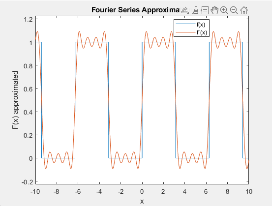
B.2) Using the command hold on, plot the graph produced by CODE 1 and CODE 2 on the same picture. Consider the number of terms N_TERMS = 7. Insert a legend on your plot describing the two signals: name the ideal square wave f(x) and the approximation f’(x).

B.3) Run the code that results from B.2 for N_TERMS = 10,20 and 30 without closing the Figure each time you run. This way you will have multiple plots on Figure 1. Include the plot on your report and answer the following question: considering the ideal square wave f(x) as a reference, where in the signal wave do the approximations of f(x) have the greatest error/oscillation? 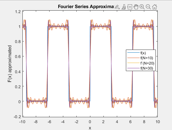When looking at he resulting waves it is plain to see that the greatest error occurs when the wave needs to make the jump to one. After this point the line is straight and the sine waves can get pretty close to a constant value.

B.4) The Gibbs phenomenon is an overshoot (or "ringing") of the Fourier series. Defining the overshoot as the difference in amplitude between the highest point of the approximation and the reference function, record the overshoot values in Table 1 associated with each of the following number of terms. What is the relationship between the overshoot and the number of terms in the series?
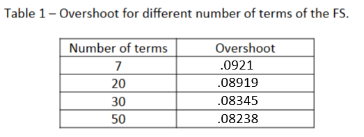The overshoot seems to decrease as the number of terms increases. These values were recorded measuring the highest point of the approximation and the reference function. The overshoot is the difference between these two values.

B.5) Run CODE 2 multiple times (for N_TERMS = 7,20,30,50 and 100.) and, using the command tic toc, record in Table 2 the time MATLAB takes to perform the approximation of f(x). Notice that you can uncomment % tic and % toc to perform the required task. Table 2 – Computational time for different number of terms of the FS. 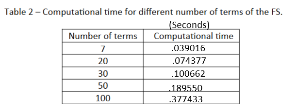The above table shows how the computational time increases as the number of terms increases.

B.6) From the previous problems it could be noticed that, the higher number of terms of the series is, more precise the approximation will be; however, the computational time cost increases. In practice, we must find a balance between precision and computational cost when using Fourier series. What determines this balance?
The balance is determined by the application of the fourier series. If a very precise answer is needed then the computational time is worth it. However, if the application is not as precise then the computational time is not worth it. These two factors must be traded off to get the best result and is completely based off what type of system is being used. If the system is a very complex periodic system then the computational time is worth it. However, if the system is a simple square wave then the computational time is not worth it.

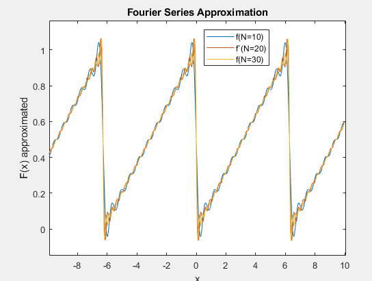
C.1) CODE 2 implements the approximation of a square wave using Fourier series. Modify this code so that it will produce the approximation of a triangular wave (more specifically, a sawtooth wave) similar to the one shown in Figure 1. In your report, include, on the same figure, plots of the approximated sawtooth function considering N_TERMS = 10,20 and 30.

Conclusion

What did you enjoy about this lab?
I really enjoyed this lab and making a fourier series in matlab. It was cool to see how the square wave can be approximated so easily. The sound portion was interesting as well and goes ot show the complexities of sound engineering.
What didn’t go well in this lab?
I did not realize that the first part of this lab was going to make noise and it was very loud with earphones on :o
How would you improve the lab experiment for future classes?
I would add mmaybe a live script to be able to actively interact with the fourier series.

Lab Report - Lab 10: Fourier Series Matlab

Introduction

Procedures

Conclusion

Code